Primer to Scale-invariant Feature Transform
Scale-invariant Feature Transform, also known as SIFT, is a method to consistently represent features in an image even under different scales, rotations and lighting conditions. Since the video series by First Principles of Computer Vision covers the details very well, the post covers mainly my intuition. The topic requires prior knowledge on using Laplacian of Gaussian for edge detection in images.
Why extract features?
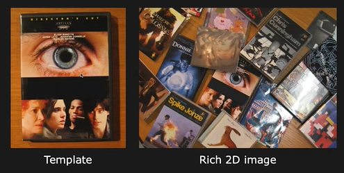 Image by First Principles of Computer Vision
Consider the two images. How can the computer recognize that the object in the left is included inside the image on the right? One way is to use template-based matching where the left image is overlapped onto the right. Then some form of similarity measure can be calculated as it is shifted across the right image.
Problem: To ensure different scales are accounted for, we would need templates of different sizes. To check for different orientations, we would need a template for every unit of angle. To overcome occlusion, we may even need to split the left image into multiple pieces and check if each of them matches.
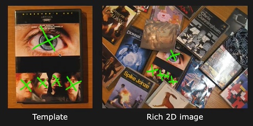
For the example above, our brains recognize the eye and the faces to locate the book. Our eyes do not scan every pixel, and we are not affected by the differences in scale and rotation. Similarly it will be great if we can 1) extract only interesting features from an image and 2) transform them into representations that are consistent across different scenes.
Good requirements for feature representation
Points of Interest: Blob-like features with rich details are preferred over simple corners or edges.
Insensitive to Scale: The feature representation should be normalized to its size.
Insensitive to Rotation: The feature representation should be able to undo the effects of rotation.
Insensitive to Lighting: The feature representation should be consistent under different lighting conditions.
Blob detection - Scale-normalized points of interest
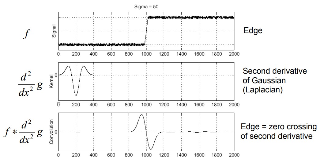 Image from Princeton CS429 - 1D edge detection
In traditional edge detection, a Laplacian operator can be applied to an image through convolution. Edges can be identified from the ripples in the response.
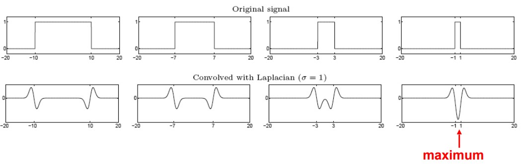 Image from Princeton CS429 - 1D blob detection
If multiple edges are at the right distance, there will be a single strong ripple caused by constructive interference. If this response is sufficiently strong, the location is identified as a blob representing a feature. Intuitively, complex features will be chosen compared to simple edges as constructive interferences cannot be produced by single edges.
From the same diagram, we can also see that not all collection of edges result in singular ripples with a particular Laplacian operator. By increasing the sigma (σ) of the Laplacian (making the kernel “fatter”), the constructive interference will occur when edges are further apart. If we apply the Laplacian operators many times with varying σ’s, blobs of different scales can be identified each time.
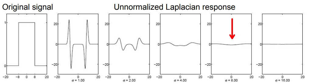 Image from Princeton CS429 - Increasing σ to identify larger blobs
Wait but if the σ is larger, the Laplacian response will be weaker (shown above). Intuitively, if the responses by larger blobs are penalized for their sizes. Does that means the selected features will be mostly tiny?
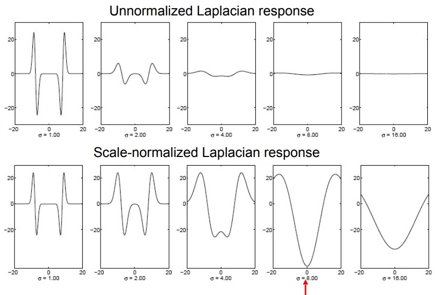 Image from Princeton CS429 - Normalized Laplacian of the Gaussian (NLoG)
We solve this by multiplying the Laplacian response with σ2 for normalization. (This works out because the Laplacian is the 2nd Gaussian derivative) Intuitively, this means that the response now only indicates the complexity of the features without any effect from their sizes.
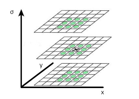 3 x 3 x 3 kernels to find local extremas
Imagine the Laplacian response represented as a matrix with x-y plane for image dimensions and z axis for various σ. We can slide an n x n x n kernel to find the local extremas. The resulting x-y coordinates would represent the centers of the blobs and σ would correspond to their sizes.
With this technique, blobs can be extracted to represent complex features with the sizes normalized.
Countering the effects of rotation
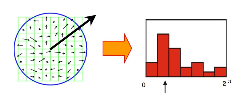 Image from Princeton CS429
To assign an orientation to each feature, it can be divided into smaller windows as shown above. Then the pixel gradient for each window can be computed to produce a histogram of gradient directions. The most prominent direction can be assigned as the principle orientation of the feature.
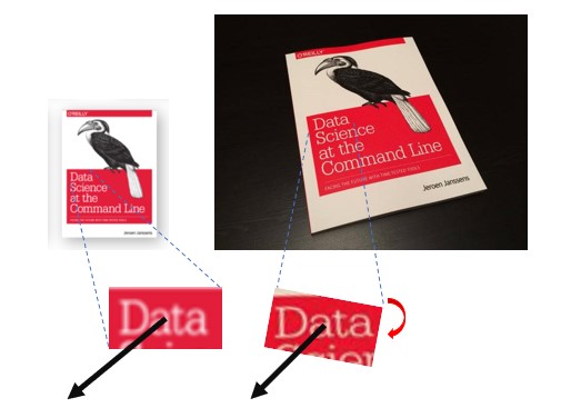 Image by Author
In the example above, blobs are identified in both images representing the same feature. The black arrows are the principle orientations. After rescaling the blob sizes with the corresponding σ’s, the effect of rotation is eliminated by aligning with respect to the principle orientations.
Countering the effects of lighting conditions
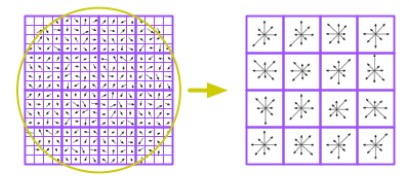 Image from Princeton CS429 - Pixels to SIFT descriptors
Instead of comparing each blob directly (pixel-by-pixel), we can produce a unique representation that is invariant to lighting conditions. As shown above, the image can be broken into smaller windows (4 x 4) where each histogram of the gradients is computed. If each histogram only consider 8 directions, there will be 8 dimensions per window. Even with only 16 windows per blob, each feature representation will be of 128 dimensions (16 x 8) which can be robust.
These feature representations are known more formally as SIFT descriptors.
Conclusion
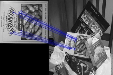 Image from OpenCV documentation
For matching images, SIFT descriptors in two images can be directly compared against one another through similarity measurements. If a large number of them matches, it is likely that the same objects are observed in both images. In practice, nearest neighbor algorithms such as FLANN are used to match the features between images.